|
 |
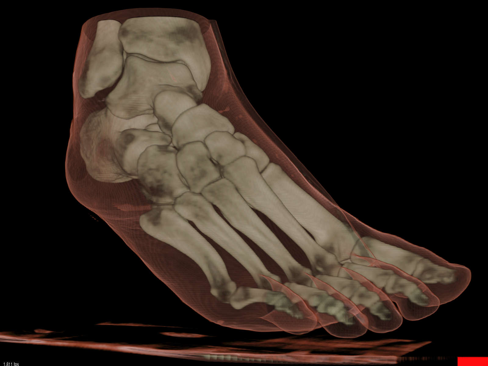
Volume rendering of a CT of a foot. Left: Trilinear interpolation of original data set (183 x 255 x 125 voxels). Right: Trilinear interpolation of supersampled data set (365 x 509 x 249 voxels). The used reconstruction filter was a 5-lobe Lanczos filter. Both images, as shown, rendered at 0.5 fps and 0.49 fps for the low and high quality versions, respectively. |
 |
 |
 |
 |
 |
 |
Volume rendering of a CT of part of an engine. Left: Trilinear interpolation of original data set (128 x 256 x 256 voxels). Right: Trilinear interpolation of supersampled data set (255 x 511 x 511 voxels). The used reconstruction filter was a 5-lobe Lanczos filter. Both images, as shown, rendered at 0.435 fps and 0.431 fps for the low and high quality versions, respectively. |
 |
 |
 |
 |
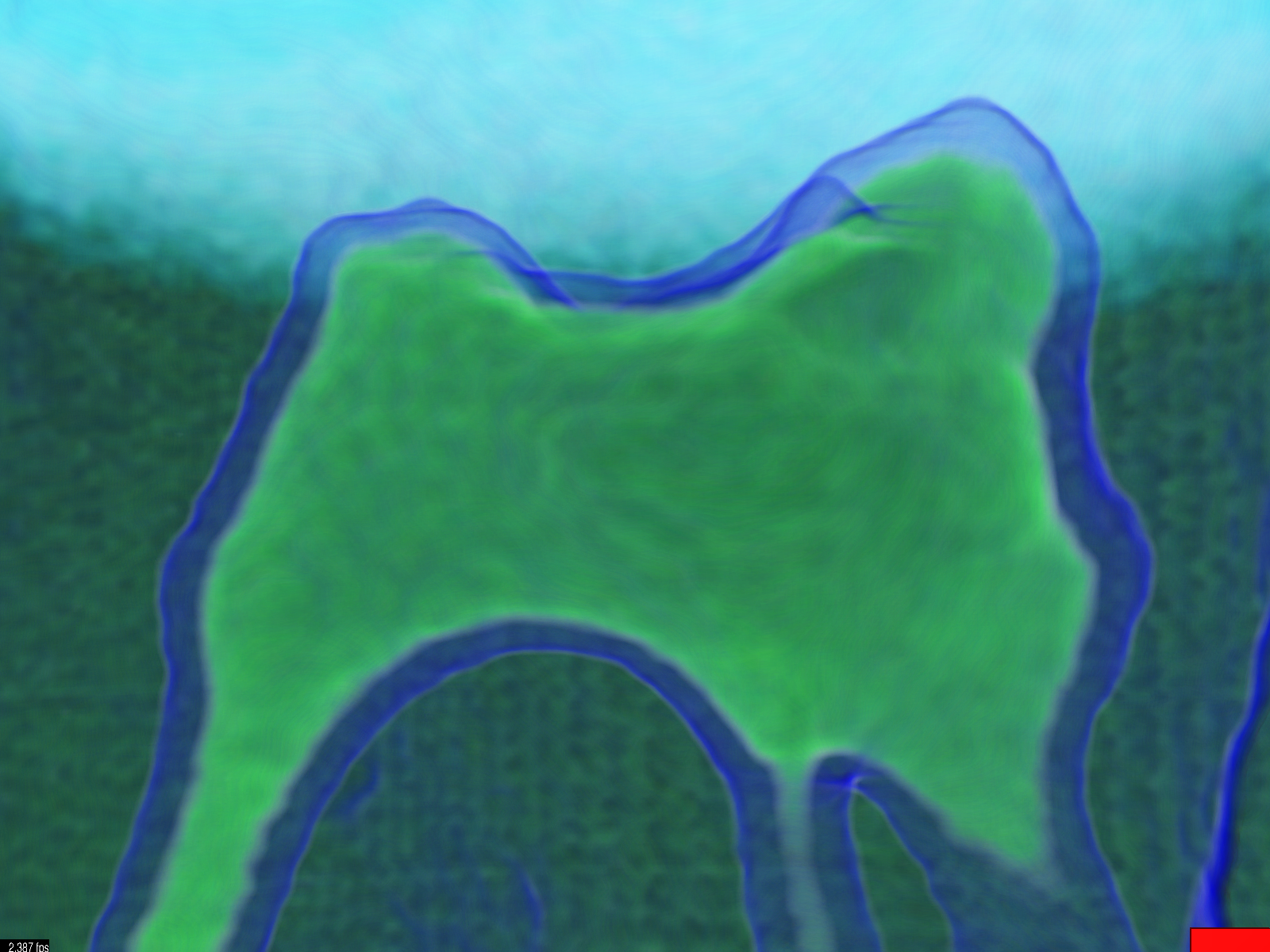
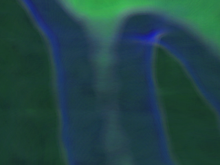
Close-up volume rendering of a CT of a tooth, showing the pulp. Left: Trilinear interpolation of original data set (160 x 256 x 256 voxels). Right: Trilinear interpolation of supersampled data set (319 x 511 x 511 voxels). The used reconstruction filter was a 5-lobe Lanczos filter. Both images, as shown, rendered at 0.292 fps and 0.291 fps for the low and high quality versions, respectively.
The detail images show an important feature (the pulp connecting to the nerve) on the scale of the voxel size. In the low-quality image, the structure is lost due to trilinear artifacts, whereas the structure is much more highly resolved in the image on the right. |
 |
 |
 |
 |
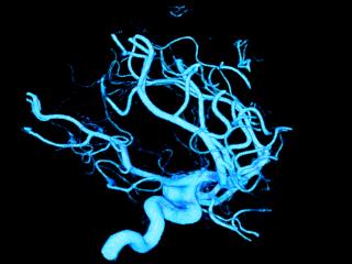
Volume rendering of a CT of a brain aneurism. Left: Trilinear interpolation of original data set (256 x 256 x 256 voxels). Right: Trilinear interpolation of supersampled data set (511 x 511 x 511 voxels). The used reconstruction filter was a 5-lobe Lanczos filter. Both images, as shown, rendered at 0.6 fps and 0.6 fps for the low and high quality versions, respectively.
The detail images show how a better reconstruction filter especially improves the fidelity of rendering small features on the scale of voxel size. |
 |
 |
 |
 |
 |
 |
Marching Cubes isosurface of the artificial Marschner-Lobb function. The function was sampled on a 41 x 41 x 41 grid of 8-bit voxels, and exhibits frequency components just below the Nyquist limit. The isosurface on the left was extracted directly from the sampled data, whereas the isosurface on the right was extracted after upsampling the original data by a factor of 4 in each direction, using a 7-tap Lanczos reconstruction filter. The image on the right shows the high-frequency components with much higher fidelity. The artifacts in the middle of the low-frequency component are due to quantization errors in the original data. |