Modeling and Data Analysis in Life Sciences: 2017

Lab4: Clustering

The following hands-on exercises were designed to teach you step by step how to perform and understand various clustering algorithm. We will look at two standard data sets: the Fisher data set on irises, and a gene expression dataset related to lung cancers.

Handouts

Exercise 1: Clustering the Fisher iris data set

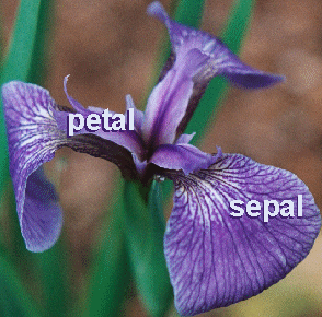
In the 1920's, botanists collected measurements on the sepal length and width, and on the petal length and width of 150 irises, 50 from each of three species (setosa, versicolor, virginica) The measurements became known as Fisher's iris data

1. Statistics on the Fisher iris dataset

   Load the Fisher iris data set:

   
   >> load fisheriris
   
   

   Note that this will create two arrays:

   • species: gives the species of each iris considered (of size 150):
     

     
     >> species(1:5)
     
     ans = 
     
         'setosa'
         'setosa'
         'setosa'
         'setosa'
         'setosa'
     
     >> species(145:150)
     
     ans = 
     
         'virginica'
         'virginica'
         'virginica'
         'virginica'
         'virginica'
         'virginica'
     
     

   • meas: matrix of size 150x4, that gives the four measurements for each iris (in the order sepal length, sepal width, petal length, petal width).

     
     >> meas(1:4,1:4)
     
     

     	Sepal length	Sepal width	Petal length	Petal width
     iris1	5.1000	3.5000	1.4000	0.2000
     iris2	4.9000	3.0000	1.4000	0.2000
     iris3	4.7000	3.2000	1.3000	0.2000
     iris4	4.6000	3.1000	1.5000	0.2000

   You will:

   1. Create three data arrays, setosa, versicolor, and virginica, that are specific to each iris species
   2. Compute the statistics (mean, standard deviation) for each measurement, for each iris species. Which two measures have the highest correlation coefficients (for each specie)? Fill up the table:
      
      

      	Setosa			Versicolor			Virginica
      Measure	Mean	Std. Deviation	Best correlation	Mean	Std. Deviation	Best correlation	Mean	Std. Deviation	Best correlation
      Sepal length
      Sepal width
      Petal length
      Petal width

   
   
   3. Generate on a single page 6 subplots, each showing the values of two characteristics of the irises, for all three types of irises. For example, the first subplot will have “Sepal length” as X axis and “Sepal Width” as Y axis, with Setosa in red, Versicolor in green, and Virginica in blue.
   
   
2. Clustering
   
   

   We go back to the full measurement array, meas. We will cluster the 150 irises into 3 clusters, and compare the results with the actual species of these 150 irises.

   There are (at least) two cluster methods implemented in Matlab:
   • Hierarchical clustering: use the function clusterdata. The basic syntax for this function is:

     
     idx = clusterdata(meas,'distance',dist_method,'linkage', link_method,'maxclust',Nclust)
     
     

     where:
     • 'distance' specifies the method used to measure the similarity of two measurements. Standard values for 'Distance' are 'euclidean','correlation', 'cosine'
     • 'linkage' specifies the linkage method used to compute the distance between two clusters. Standard methods include 'single','average', and 'complete'.
     • 'maxclust' is the number of clusters expected
     • 'idx' is the array of cluster assignment for each data point (in our case, irises), after clustering.
     
     For example,

     
     Idx = clusterdata(meas,'distance','euclidean','linkage', 'single','maxclust',3)
     
     

     will cluster the data using the Euclidian distance to compare data points, single linkage to compare clusters, and output 3 clusters.
   
   
   • kmeans clustering: use the function kmeans. The basic syntax for the function is:
     

     
     idx = kmeans(meas,K,'Distance',dist_method)
     
     

     where:
     • K is the number of clusters
     • 'Distance' specifies the method used to measure the similarity of two measurements. Standard values for 'Distance' are 'sqEuclidean','correlation', 'cosine'
     • 'idx' is the array of cluster assignment for each data point (in our case, irises), after clustering.
     
     For example,

     
     Idx = kmeans(meas,3,'Distance','correlation')
     
     

     will cluster the data using k-means, with k set to 3 clusters, and using correlation to compare data points.
   
   

   Once the irises have been clustered, we need to compare the cluster assignments of the irises with their actual species. Useful tools for this include:

   • crosstab
     crosstab(idx,species) will build a matrix C of size Ncluster x 3, with C(i,j) gives the number of elements of cluster I that belongs to specie j.
   • randindex
     R=randindex(idx,species)gives an Index of quality for the two partitioning of the data, idx (from the clustering technique), and species. Note that randindex is not a Matlab built in function. You can get it from here.

   Experiment with the different clustering techniques. Fill in this table:

   Technique	Distance	Linkage	RandIndex
   Hierarchical	Euclidean	Single
   Hierarchical	Euclidean	Average
   Hierarchical	Euclidean	Complete
   Hierarchical	Correlation	Single
   Hierarchical	Correlation	Average
   Hierarchical	Correlation	Complete
   K-means	sqEuclidean
   K-means	Correlation
   K-means	Cosine

   Which method works "best"?

   For this method, plot the silhouette for each flower, organized in clusters.

Exercise 2: Clustering the spiral dataset

Some examples:

• A simple two-cluster example: The data twocluster.crd and corresponding MATLAB script simple.m
• The eared-mouse example: The data mouse.crd and corresponding MATLAB script clustermouse.m

The spiral dataset corresponds to three intertwined spirals, each with approximately 100 points. This dataset is usually considered difficult to cluster, as each spiral is not “convex”; we will come to what it means later. You will attempt to cluster this data set using hierarchical clustering

The spiral dataset is available in the file spiral.crd. This file contains two columns, corresponding to the X and Y coordinates of the 312 data points in the dataset. Points 1 to 106 belongs to spiral 1 (red), 107 to 207 to spiral 2 (green), and 208 to 312 to spiral 3 (blue).

1. Generate a figure that resembles the figure shown above.
2. Generate on a single page 4 subplots, each showing the results of clustering the spiral dataset, using a different linkage definition. I advise that you try: 'single','average', 'complete' and 'ward'. Explain what you obtain. You may want to quantify the quality of the clustering you obtain using the function randindex.