Modeling and Data Analysis in Life Sciences: 2017

Project 3: Image processing (drawing of an elephant)

We all use Fourier analysis without even knowing it: cell phones, DVDs, images, all involve Fourier transforms in one form or another. This lab includes one exercise that illustrates the computation and interpretation of Fourier analysis for a 2D image (drawing an elephant).

Handouts

Drawing an elephant

There is a famous joke in physics that comes from a conversation between the two physicists Freeman Dyson and Enrico Fermi. As Dyson reported ("A conversation with Fermi", Nature, 427, 297 (2004)):

"In desperation I asked Fermi whether he was not impressed by the agreement between our calculated numbers and his measured numbers. He replied, "How many arbitrary parameters did you use for your calculations?" I thought for a moment about our cut-off procedures and said, "Four." He said, "I remember my friend Johnny van Neumann used to say, with four parameters I can fit an elephant, and with five I can make him wiggle his trunk." With that, the conversation was over."

Can we really draw an elephant with four parameters? The answer is yes, according to a recent paper by Howard and colleagues (Mayer et al, "Drawing an elephant with four complex parameters", Am. J. Phys., 78, 648 (2010)). We will attempt to repeat their study in this exercise. The file elephant.jpg contains a picture of a hand-drawn elephant. (see figure).The goal is to reconstitute this drawing with an analytical function representing the elephant that has a minimal number of parameters.

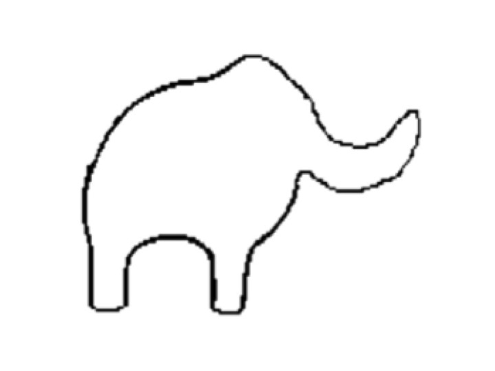
The strategy is:

1. Read the image file and generate a binary version of the image

   
   %The matlab command for reading an image file is: imread:
   
   elephant = imread('elephant.jpg')
   
   % You can visualize the image with:
   
   figure
   imshow(elephant) 
   
   % A binary version of the image can be obtained by applying a filter. 
   % For example, if the image is named 'elephant', the command:
   
   elbin = elephant < T
   
   % generates a binary image of the same size as the image elephant, 
   % with value 1 if the corresponding pixel in 'elephant' has 
   % an intensity smaller than T, and 0 otherwise.
   
   

2. Extract the contour of the elephant. The idea is to parametrize each point M of the contour in the form \(M(x(t),y(t))\), where t is a parameter that can be interpreted as the elapsed time required to draw this contour

   
   
   % A Matlab command for getting the boundary of objects included in an image is:
   
   perim = bwboundaries(elbin,4,'noholes');
   
   % Note that bwboundary will generate as many contiguous contours as there are 
   % objects in the% image. For our elephant, it should generate a single contour.
   % The output of bwboundary should be stored in two arrays X and Y:
   
   boundary = perim{1};
   %
   X = boundary(:,2);
   Y = boundary(:,1);
   
   

3. Compute the Fourier series for both X and Y:
   
   The idea is to write: $$X(t) = \sum_{k=0}^{+\infty} A_k^{x} \cos(kt) + B_k^{x} \sin(kt)$$ $$Y(t) = \sum_{k=0}^{+\infty} A_k^{y} \cos(kt) + B_k^{y} \sin(kt)$$
   

   
   % To compute the coefficients A and B for example for X, we would use 
   % the Matlab commands:
   
   N=size(X);
   C=fft(X);
   AX=real(C)/(2*N);
   BX=-imag(C)/(2*N);
   
   % Note that AX(1) and BX(1) contains information about the center of gravity 
   % of the object represented by X, and are not needed for reconstruction
   
   

4. Reconstruct the elephant with up to M coefficents:
   
   

   Once the values of AX, BX, AY, and BY have been computed, it is possible to reconstruct the image with an approximation of order M by implementing the following equations:

   $$Xr(t) = \sum_{k=0}^{M} A_k^{x} \cos(kt) + B_k^{x} \sin(kt)$$ $$Yr(t) = \sum_{k=0}^{M} A_k^{y} \cos(kt) + B_k^{y} \sin(kt)$$

   To check to quality of the approximation, just plot the result:

   
   plot(Xr,Yr,'-r')
   
   

Problem:

1. Complete and implement this program; test it on the file elephant.jpg.
2. Generate on a single page four subplots representing the approximation of the elephant you have obtained for \(M = 1, M=4, M=10\), and \(M=100\).